Units: umol/l. Method: spatial interpolation produced with DIVA (Data-Interpolating Variational Analysis). URL: http://modb.oce.ulg.ac.be/DIVA. Comment: Every year of the time dimension corresponds to a 10-year centred average for each season : - winter season (December-February), - spring (March-May), - summer (June-August), - autumn (September-November). Diva settings: Snr=1.0, CL=0.7.

Units: umol/l. Method: spatial interpolation produced with DIVA (Data-Interpolating Variational Analysis). URL: http://modb.oce.ulg.ac.be/DIVA. Comment: Every year of the time dimension corresponds to a 10-year centred average for each season : - winter season (December-February), - spring (March-May), - summer (June-August), - autumn (September-November). Diva settings: Snr=1.0, CL=0.7.

Units: umol/l. Method: spatial interpolation produced with DIVA (Data-Interpolating Variational Analysis). URL: http://modb.oce.ulg.ac.be/DIVA. Comment: Every year of the time dimension corresponds to a 10-year centred average for each season : - winter season (December-February), - spring (March-May), - summer (June-August), - autumn (September-November). Diva settings: Snr=1.0, CL=0.7

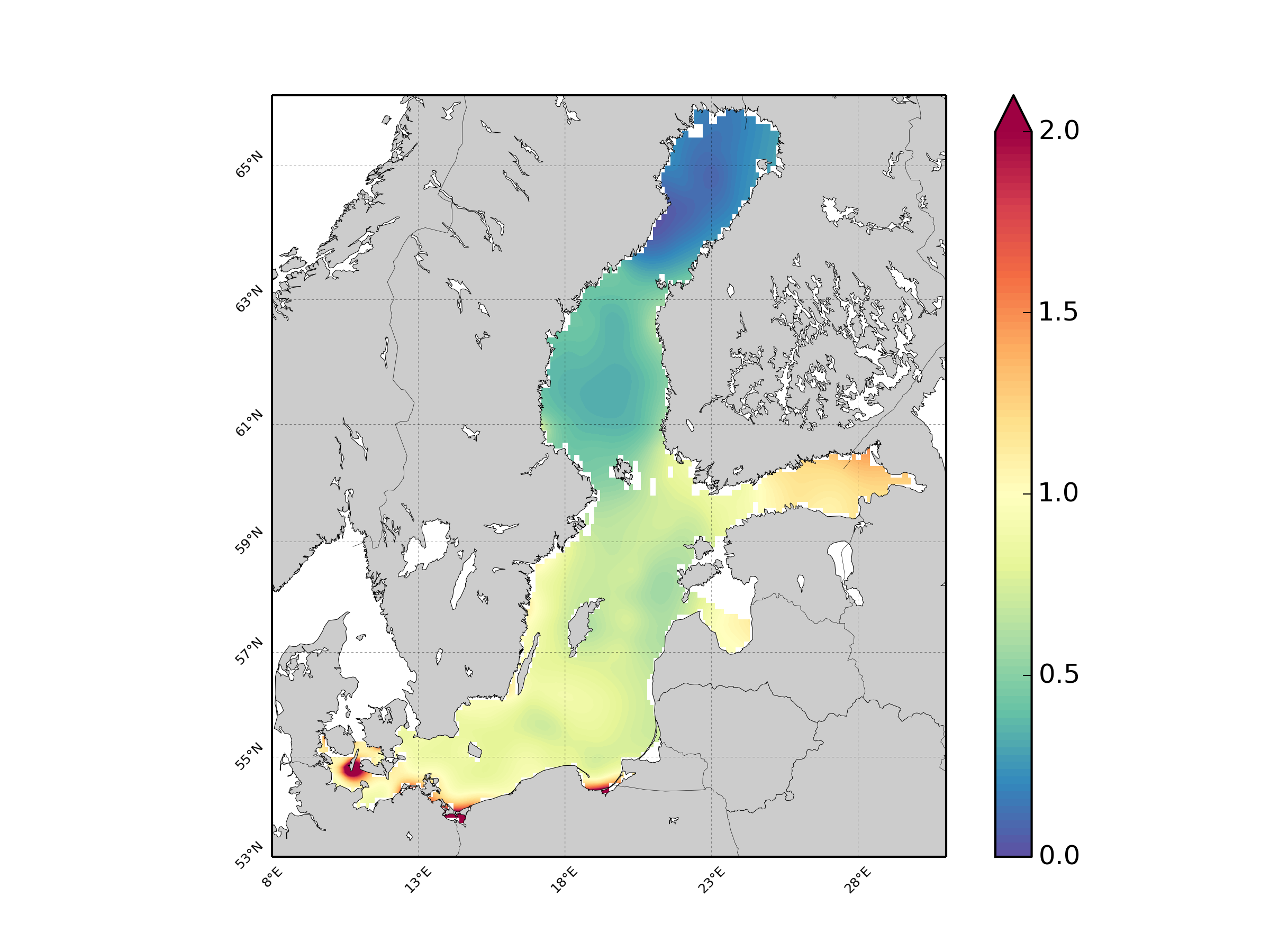
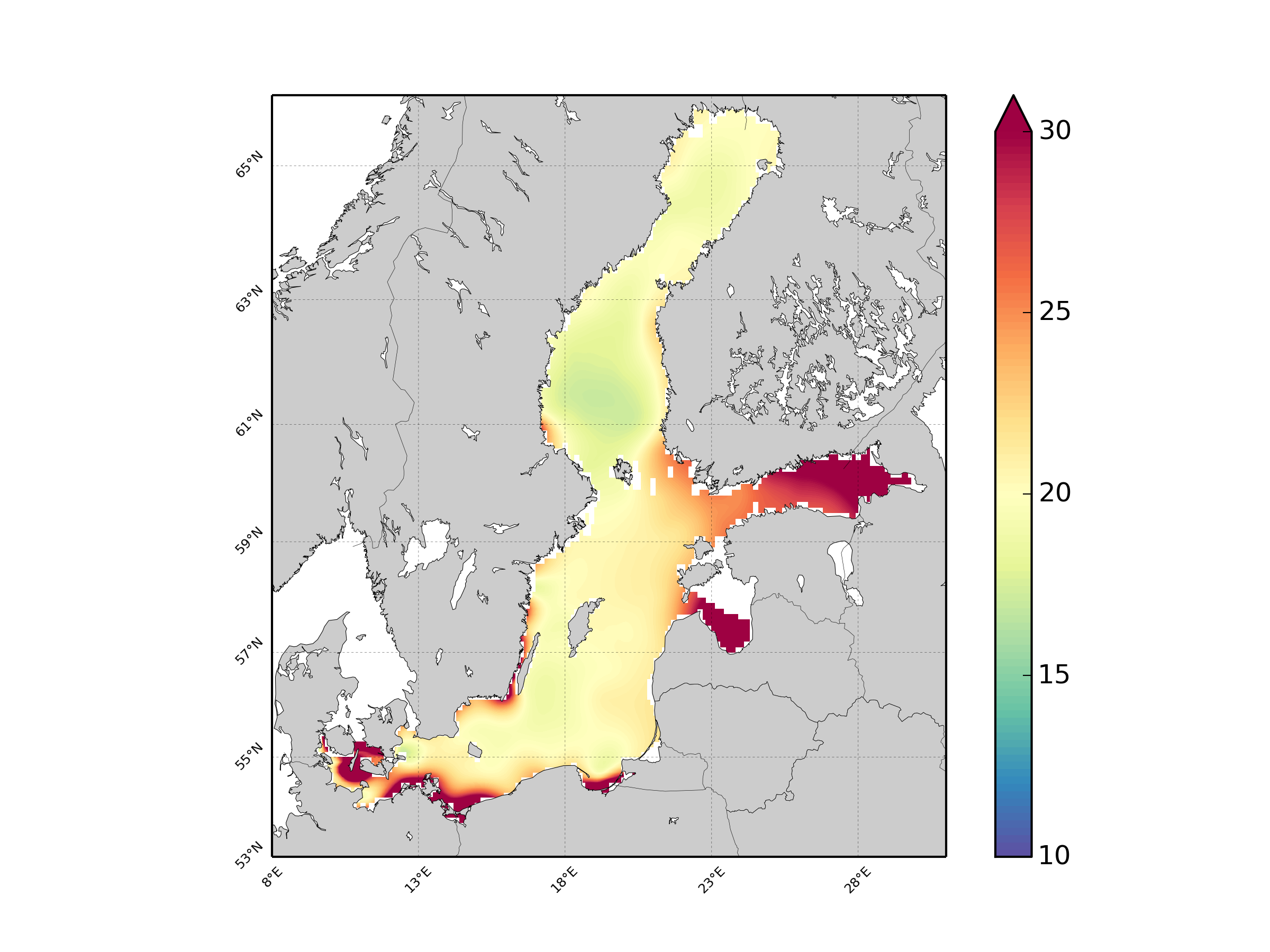
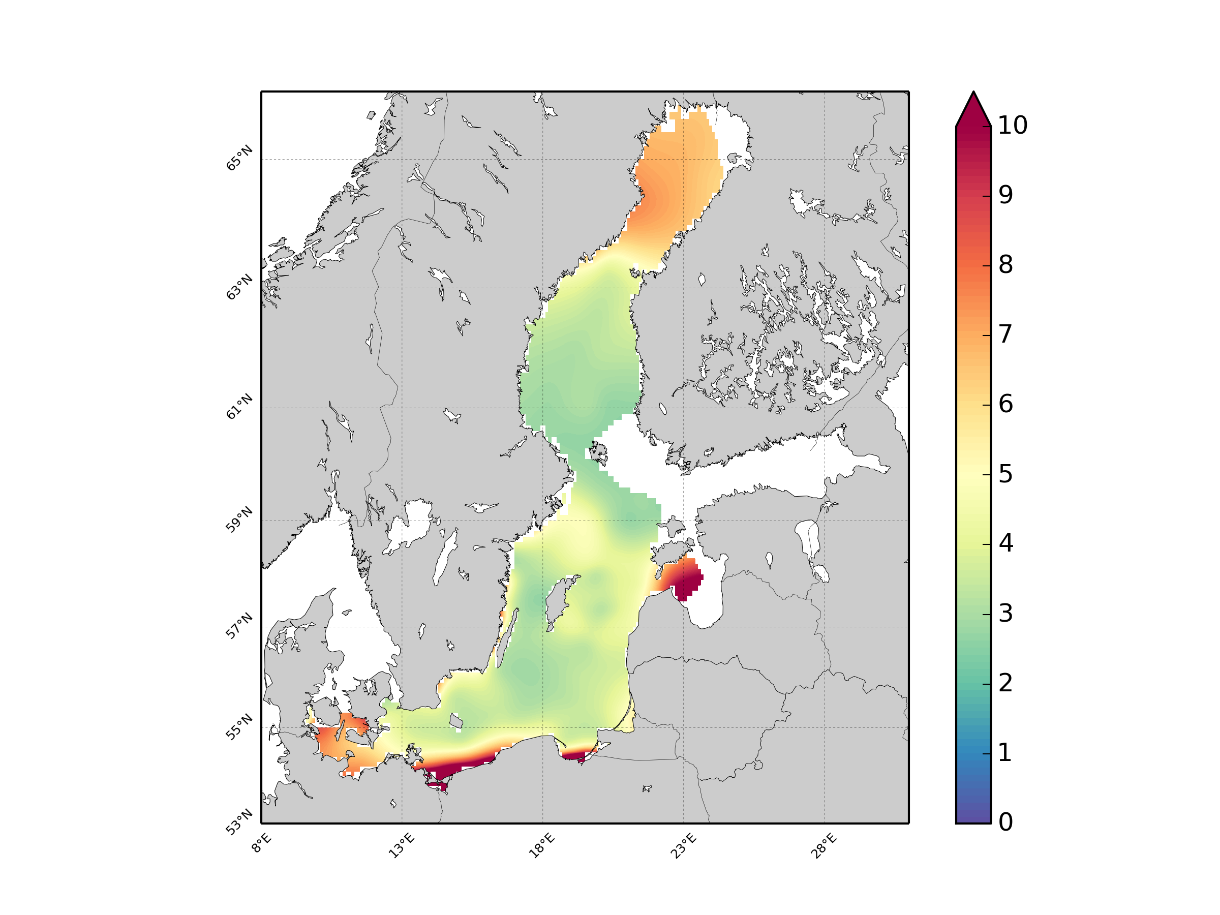
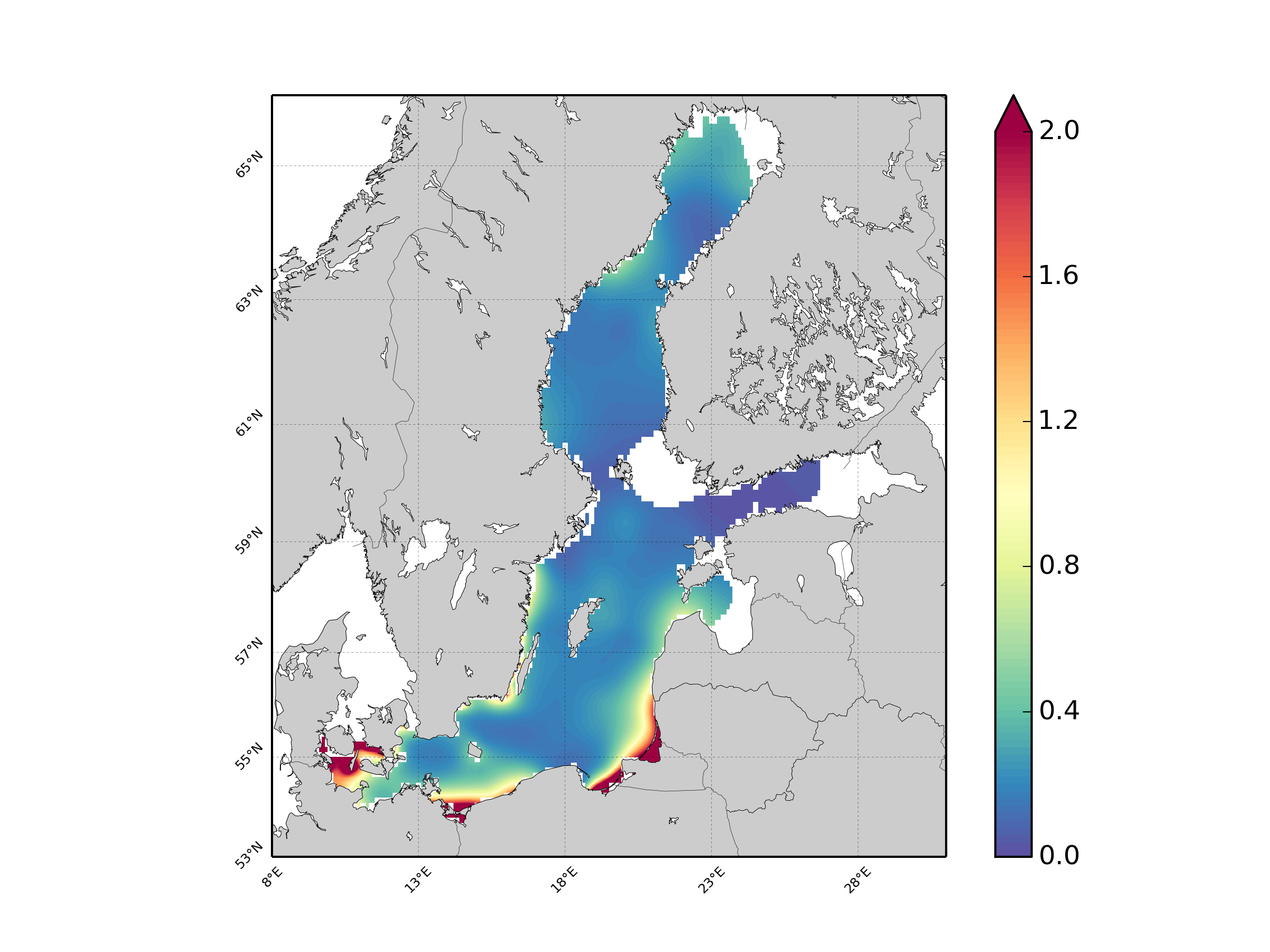
Units: umol/l. Method: spatial interpolation produced with DIVA (Data-Interpolating Variational Analysis). URL: http://modb.oce.ulg.ac.be/DIVA. Comment: Every year of the time dimension corresponds to a 10-year centred average for each season : - winter season (December-February), - spring (March-May), - summer (June-August), - autumn (September-November). Diva settings: Snr=1.0, CL=0.7

Units: umol/l. Method: spatial interpolation produced with DIVA (Data-Interpolating Variational Analysis). URL: http://modb.oce.ulg.ac.be/DIVA. Comment: Every year of the time dimension corresponds to a 10-year centred average for each season : - winter season (December-February), - spring (March-May), - summer (June-August), - autumn (September-November). Diva settings: Snr=1.0, CL=0.7.

Units: umol/l. Method: spatial interpolation produced with DIVA (Data-Interpolating Variational Analysis). URL: http://modb.oce.ulg.ac.be/DIVA. Comment: Every year of the time dimension corresponds to a 10-year centred average for each season : - winter season (December-February), - spring (March-May), - summer (June-August), - autumn (September-November). Diva settings: Snr=1.0, CL=0.7.

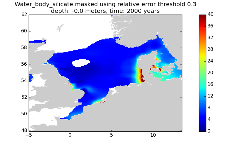
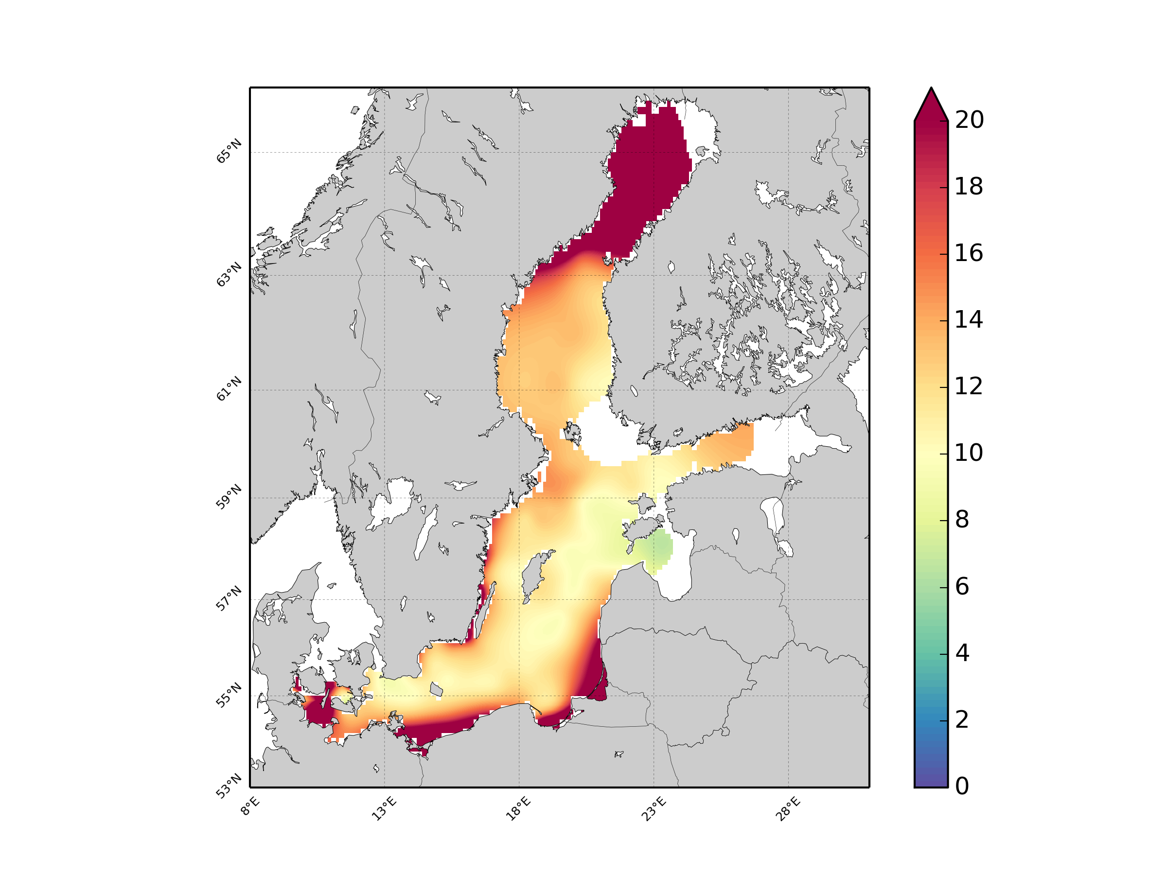
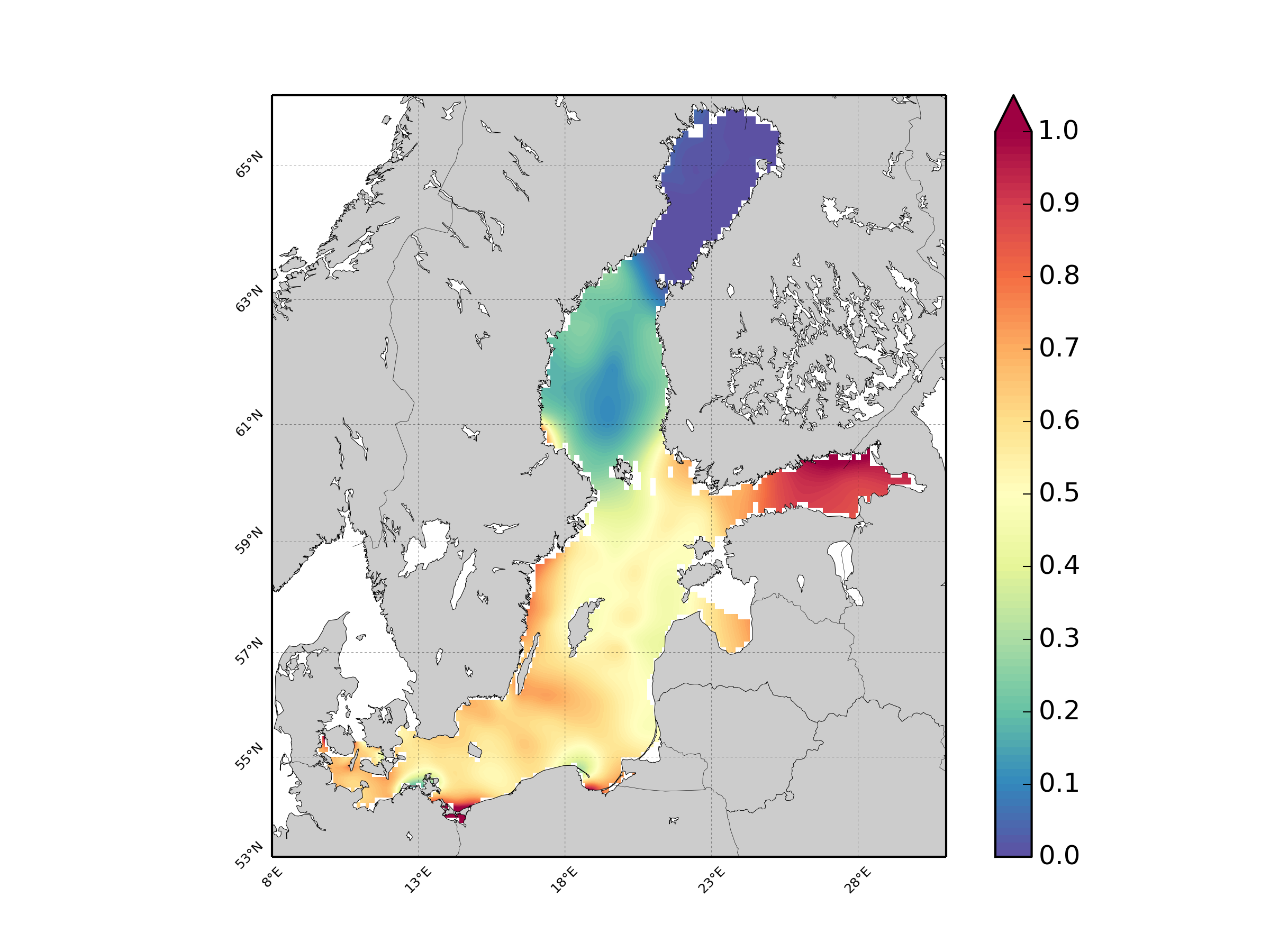
This gridded product visualizes 1960 - 2014 water body silicate concentration (umol/l) in the North Sea domain, for each season (winter: December – February; spring: March – May; summer: June – August; autumn: September – November). It is produced as a Diva 4D analysis, version 4.6.9: a reference field of all seasonal data between 1960-2014 was used; results were logit transformed to avoid negative/underestimated values in the interpolated results; error threshold masks L1 (0.3) and L2 (0.5) are included as well as the unmasked field. Every step of the time dimension corresponds to a 10-year moving average for each season. The depth dimension allows visualizing the gridded field at various depths.

<para>Phytolankton have been regionally monitored in Sweden since 1985.</para> <para>The monitoring is financed by the Swedish county administration boards, Swedish municipalities and Swedish coalitions of water conservation. Recipient control data financed by companies are also included. Monitoring is performed by Swedish universities and consulting firms.</para> <para>Data are stored in the Swedish Ocean Archive database (SHARK), by the Swedish Meteorological and Hydrological Institute. Data are collected and analyzed according to the HELCOM COMBINE Manual - Part C Annex C6 Monitoring of phytoplankton species composition, abundance and biomass (https://www.helcom.fi/wp-content/uploads/2019/08/Guidelines-for-monitoring-phytoplankton-species-composition-abundance-and-biomass.pdf) or similar methods.</para>

<para>Zoobenthos have been regionally monitored in Sweden since 1972. The monitoring is financed by the Swedish county administration boards, Swedish municipalities, Swedish coalitions of water conservation and Swedish companies. Recipient control data financed by companies are also included.</para>

Data collected within various monitoring programmes and surveys. Standard zoobenthos techniques using benthic grabbers and species analyses for counts and weights on species level.